Andrew Carr blog

Alan Kay said that Lisp is

greatest single programming language ever designed.

With all the attention it has received, it's hard to argue that Lisp is an esoteric programming language. This "LISt Processing" language has many implementations, but one main constants is that the line between code and data is blurred. This makes it a

programmable programming language.¹

The purpose of this article is not to talk about Lisp. I am not expert, and there is a vast literature on the subject from many bright minds. The true point of this post is to talk about a specific Lisp: Hylang.

Hy is a Python Lisp! It is a Lisp that is "embedded" in Python. More specifically, from the Hy homepage²

Since Hy transforms its Lisp code into the Python Abstract Syntax Tree, you have the whole beautiful world of Python at your fingertips, in Lisp form!

This means you can gain many of the benefits of a Lisp, while having access to the vast Python data science library. There are some drawbacks to this method, but in general it's an exciting and extremely satisfying little language.

To showcase some of the joy of Hy, we'll be estimating the value of π using Monte Carlo integration. This isn't necessarily a data science task, but it is an interesting bit of mathematics, and complicated enough to need some interesting code.

First, the math

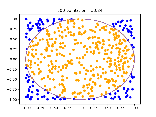
Because we know the area of a circle of radius $r$ is $A = \pi r^2$ we can estimate $\pi$ by computing the area of the unit circle. This amounts to uniformly sampling points in a certain domain around the unit circle. The percentage of points in the circle gives a good approximation of how much of the domain is taken up by the circle. We can then multiply that percentage by the total area of the domain to get an estimate for the circle's area, and thereby estimating pi.

We can do this estimate of π by formulating an integral problem, which we later discretize. We first define $f : \mathbb{R}^2 \rightarrow \mathbb{R}$ $$f(x) = \begin{cases} 1, & \text{if $||x||_2 < 1$} \\[2ex] 0, & \text{otherwise} \end{cases}$$ We then let $\Omega = [-1,1] \times [-1,1]$ be the unit square and our estimate can be obtained through $$\int_{-1}^1 \int_{-1}^1 f(x,y) dx dy = \pi$$

Now, the code

We can now start writing some Hy.

Like most Lisps, Hy has brackets galore, but after some time this syntax is quite lovely. Most imperative code we're used to seeing uses Infix notation. Lisp uses something similar to Prefix notation, but not exactly. It's truly unique.

(+ 1 1)
>2

(lfor x (range 10) (+ 3.14 x))
>[3.14, 4.14, 5.14, 6.14, 7.14, 8.14, 9.14, 10.14, 11.14, 12.14]

(setv result (- (/ (+ 1 3 88) 2) 8))
(print result)
>38.0

Lisp is a wonderful way to define recursive functions. For example, if we want to sum a list, we could write a function that takes in a list, checks the base case for an empty list, then adds the first element with the sum of the rest of the list.

(defn sum_li [li]
(cond 
    [(empty? li) 0
        (0)]
    [(= (len li) 1)
        (first li)]
    [True
        (+ (first li) (sum_li (list (rest li))))]
))
(print (sum_li [1, 2, 3, 4, 5]))
>15
                

Or, since we're really writing in Python, we can use built-in functions

(sum [1, 2, 3, 4, 5])
>15

I think we're ready to dive into our Hy Monte Carlo estimation. We start with some basic imports

(import [numpy :as np])
(import [scipy.linalg :as la])
(import [matplotlib.pyplot :as plt]

We then define our function monte_estimate which takes in a value n and returns an estimate for $\pi$

(defn monte_estimate [n]
(setv points (np.random.uniform -1 1 :size [2 n]))
(setv lengths (la.norm points :axis 0))
(setv num_within 
    (np.count_nonzero 
        (< lengths 1)
    )
)
(setv out (* 4 (/ num_within n))
)

There is a lot to unpack here.

We start the function by sampling random points in the unit square.

(setv points (np.random.uniform -1 1 :size [2 n]))

We then get the distance of each point from the center

(setv lengths (la.norm points :axis 0))

We count the number of lengths that are within the unit circle (less than 1). We multiply and divide to get an estimate of $\pi$

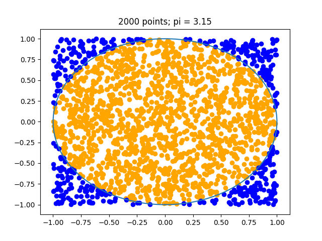
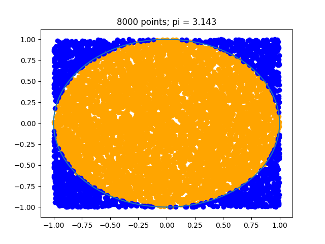
In the case of n = 500 we can an estimate of around $3.12$ or $3.024$ as in the below. As we increase $n$ the estimate will improve.

These plots were also created in Hy, they required use of macros to recreate the slicing ability of numpy. Below is the code for the interested.

(import [numpy :as np])
(import [scipy.linalg :as la])
(import [matplotlib.pyplot :as plt])

(defn parse-colon [sym]
(list (map (fn [x]
                (if (empty? x)
                    None
                    (int x)))
            (.split (str sym) ":"))))

(defn parse-indexing [sym]
(cond
    [(in ":" (str sym)) `(slice ~@(parse-colon sym))]
    [(in "..." (str sym)) 'Ellipsis]
    [True sym]))

(defmacro nget [ar &rest keys]
`(get ~ar (, ~@(map parse-indexing keys))))

(defn monte_estimate [n]
(setv points (np.random.uniform -1 1 :size [2 n]))
(setv X (np.linspace (- np.pi) np.pi 100))
(setv lengths (la.norm points :axis 0))
(setv num_within 
    (np.count_nonzero 
        (< lengths 1)
    )
)
(setv out (* 4 
            (/ num_within n)
            )
)
(plt.plot 
    (np.sin X)
    (np.cos X)
)
(setv inner_mask (< lengths 1))
(setv outer_mask (>= lengths 1))
(print (np.shape (nget (.transpose points) inner_mask 0)))
(plt.scatter (nget (.transpose points) inner_mask 0) 
                (nget (.transpose points) inner_mask 1) :color "orange")
(plt.scatter (nget (.transpose points) outer_mask 0) 
                (nget (.transpose points) outer_mask 1) :color "blue")
(plt.title f"{n} points; pi = {out}")
(plt.savefig f"{n}out.png")
(plt.clf)
(plt.close)
out)

(setv n 500)
(print (monte_estimate n))

¹John Foderaro

²Hylang Website