Data Exploration in J
When trying to answer questions that provide value to your organization, one of the first steps is collecting and exploring the data.
In this article, we have a data set with the following columns.
columns df
┌─┬───────┐
│0│id     │
├─┼───────┤
│1│dataset│
├─┼───────┤
│2│x      │
├─┼───────┤
│3│y      │
└─┴───────┘
The values are split into a few difference clusters that are labeled "I - IV" in the dataset column.
counter 1 col df
┌───┬──┐
│I  │11│
├───┼──┤
│II │11│
├───┼──┤
│III│11│
├───┼──┤
│IV │11│
└───┴──┘
5 head df
┌──┬───────┬────┬────┐
│id│dataset│x   │y   │
├──┼───────┼────┼────┤
│0 │I      │10.0│8.04│
├──┼───────┼────┼────┤
│1 │I      │8.0 │6.95│
├──┼───────┼────┼────┤
│2 │I      │13.0│7.58│
├──┼───────┼────┼────┤
│3 │I      │9.0 │8.81│
└──┴───────┴────┴────┘
┌─┬─┬────┬────┬──┬──┬────┬────┬──┬───┬────┬─────┬──┬──┬───┬────┐
│0│I│10.0│8.04│11│II│10.0│9.14│22│III│10.0│7.46 │33│IV│8.0│6.58│
├─┼─┼────┼────┼──┼──┼────┼────┼──┼───┼────┼─────┼──┼──┼───┼────┤
│1│I│8.0 │6.95│12│II│8.0 │8.14│23│III│8.0 │6.77 │34│IV│8.0│5.76│
├─┼─┼────┼────┼──┼──┼────┼────┼──┼───┼────┼─────┼──┼──┼───┼────┤
│2│I│13.0│7.58│13│II│13.0│8.74│24│III│13.0│12.74│35│IV│8.0│7.71│
├─┼─┼────┼────┼──┼──┼────┼────┼──┼───┼────┼─────┼──┼──┼───┼────┤
│3│I│9.0 │8.81│14│II│9.0 │8.77│25│III│9.0 │7.11 │36│IV│8.0│8.84│
├─┼─┼────┼────┼──┼──┼────┼────┼──┼───┼────┼─────┼──┼──┼───┼────┤
│4│I│11.0│8.33│15│II│11.0│9.26│26│III│11.0│7.81 │37│IV│8.0│8.47│
└─┴─┴────┴────┴──┴──┴────┴────┴──┴───┴────┴─────┴──┴──┴───┴────┘
If you're curious about the definitions of columns, head, counter see my previous post here
I split up the data frame based on the dataset label and then look at some descriptive statistics.
We first look at the mean values for x and y for each of the 4 data sets
┌───┬───┐
│9.4│8.9│
├───┼───┤
│8.9│9.1│
└───┴───┘
┌─────┬─────┐
│7.683│7.337│
├─────┼─────┤
│7.504│7.593│
└─────┴─────┘
Then the standard deviation for x and y
┌───────┬───────┐
│3.20416│3.47851│
├───────┼───────┤
│3.47851│3.47851│
└───────┴───────┘
┌───────┬───────┐
│2.04465│2.06347│
├───────┼───────┤
│2.14021│2.11607│
└───────┴───────┘
Fascinatingly we see that all 4 datasets have extremely similar descriptive statistics. This is surprising, and something seems a bit off. If we run a full dstat on the datasets, we begin to see some difference between the datasets.
Descriptive statistics for X values
┌───────────────────────┬───────────────────────┐
│sample size:         10│sample size:         10│
│minimum:              4│minimum:              4│
│maximum:             14│maximum:             14│
│median:             9.5│median:             8.5│
│mean:               9.4│mean:               8.9│
│std devn:       3.20416│std devn:       3.47851│
│skewness:     _0.169188│skewness:     0.0881543│
│kurtosis:       1.97835│kurtosis:       1.65537│
├───────────────────────┼───────────────────────┤
│sample size:         10│sample size:       10  │
│minimum:              4│minimum:            8  │
│maximum:             14│maximum:           19  │
│median:             8.5│median:             8  │
│mean:               8.9│mean:             9.1  │
│std devn:       3.47851│std devn:     3.47851  │
│skewness:     0.0881543│skewness:     2.66667  │
│kurtosis:       1.65537│kurtosis:     8.11111  │
└───────────────────────┴───────────────────────┘
Descriptive statistics for Y values
┌───────────────────────┬──────────────────────┐
│sample size:         10│sample size:        10│
│minimum:           4.26│minimum:           3.1│
│maximum:          10.84│maximum:          9.26│
│median:            7.81│median:           8.12│
│mean:             7.683│mean:            7.337│
│std devn:       2.04465│std devn:      2.06347│
│skewness:     _0.260857│skewness:     _1.01039│
│kurtosis:       2.35098│kurtosis:      2.74257│
├───────────────────────┼──────────────────────┤
│sample size:       10  │sample size:       10 │
│minimum:         5.39  │minimum:         5.25 │
│maximum:        12.74  │maximum:         12.5 │
│median:          6.94  │median:         7.375 │
│mean:           7.504  │mean:           7.593 │
│std devn:     2.14021  │std devn:     2.11607 │
│skewness:     1.51232  │skewness:     1.14784 │
│kurtosis:     4.65251  │kurtosis:     3.95088 │
└───────────────────────┴──────────────────────┘
By just looking at these values, it seems that each dataset is distributed very similarly. Let's do a simple linear regression and see if we can fit the data differently given the variance in skew and kurtosis.
We hope to solve an equation of the following form.
$$AX = B$$
Where $A$ is a matrix of our x values, augmented with a column of 1's to account for an intercept term.
$B$ on the other hand, is a vector of our y values.
We'll first write two monadic verbs to get these matrices for an arbitrary dataset.
get_A =: 3 : '((# (2 col y)) # 1) ,. (2 col y)'
get_B =: 3 : '3 col y'
The get_B verb is straight forwardly selecting the proper column. However, get_A is a little more complicated.
Since J is read from right to left, we'll start that way in breaking this verb apart. (2 col y) selects the $2^{nd}$ column which is then concatenated column wise via ,. with a vector of 1's of the length of our column. # (2 col y) gets an integer length and the dyad x # y repeats y, x times.
So for the first dataset, our $A$ matrix looks like the following.
get_A df1
1 10
1  8
1 13
1  9
1 11
1 14
1  6
1  4
1 12
1  7
We now write a regression verb (no longer using a one-line syntax) that solves for $X$.
reg =: 3 : 0
    A =: get_A y
    B =: get_B y
    X =: B %. A
    X
)
We can then get the intercept and slope values from the regression for each dataset. Fascinatingly, they are all extremely similar.
reg df1
> 2.90182 0.508636
reg df2
> 2.9894 0.488494
reg df3
> 3.00791 0.505179
reg df4
> 3.08253 0.495657
At this point in the data exploration process, things are starting to get a little weird. The descriptive statistics of each dataset, along with the regression coefficient unintuitively imply that each of the 4 datasets is very similar.
Let's write a verb that plots the regression line on top of a scatter plot of the actual data.
plot_quartet =: 4 : 0
    pd 'reset'
    pd 'type line'
    pd ((1 { y) * i. 20) + (0 { y)
    pd 'pensize 3.5; type point'
    pd (2 col x);(3 col x)
    pd 'show'
)
df1 plot_quartet (reg df1)
df2 plot_quartet (reg df2)
df3 plot_quartet (reg df3)
df4 plot_quartet (reg df4)
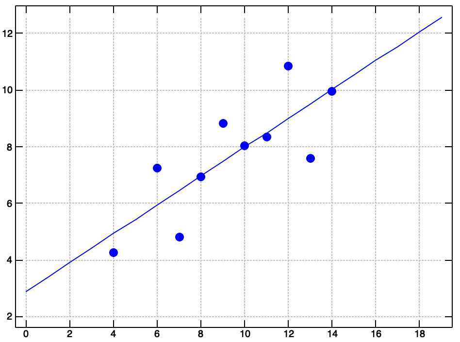
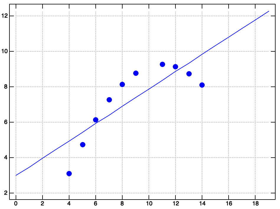
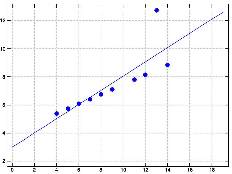
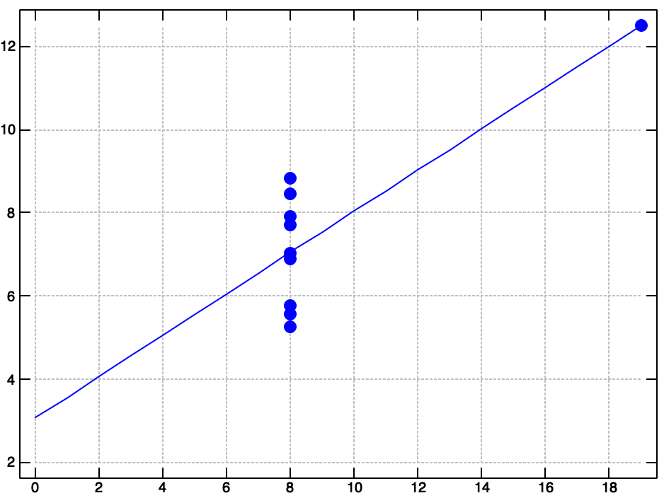
Well, there you have it. Anscombe's Quartet. Many common data exploration methods failed to reveal the strange shape of this dataset. Be careful out there! Data is slippery, and you can't always trust your first impressions.